3. Description
3.1. aXe Hierarchy
There exist two classes of aXe tasks, see figure 1).
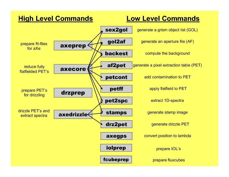
Figure 1: The list of aXe tasks.
The Low-Level Tasks work on individual grism images. All input and output refers to a particular grism image.
The High-Level Tasks work on data sets. Their aim is to perform a series of processing steps for a set of images.
The High-Level Tasks often use the Low-Level Tasks to do a certain reduction step on each frame (see figure 1 ).
The High-Level Tasks were designed to cover all steps of the aXe reduction without any restriction in functionality. All tasks are controlled through a set of configuration files , which can be edited by the user and optimized for a given data set.
3.2. Slitless Spectroscopy
In conventional spectroscopy, slits or masks are used to allow only the light from a small portion of the focal plane of the telescope to enter the dispersing device (e.g. grism, grating or prism). This results in an unambiguous conversion between pixel coordinates on the detector and wavelength.
In slitless spectroscopy there is no unique correspondence between pixel coordinates and wavelength. Consequently, the spectral reduction on the basis of the spectroscopic data alone is very difficult. Additional information concerning the positions of the object must be added to facilitate the spectral reduction. In aXe this is done by providing an Input Object List (IOL) at the beginning of the reduction process. In the Input Object List the object positions are given in the image-coordinate system or the world coordinate system. This allows the determination of the so called reference pixel for every object. The reference pixel is the undispersed object position in image coordinates on the grism data. For each individual object, it is then possible to assign a wavelength to each pixel.
In conventional spectroscopy the extraction of the 1D spectra from the 2D data is done along the direction of the slit or mask. In slitless spectroscopy, such a predefined extraction direction does not exist. It is in fact possible to define a different extraction direction for each object individually by adjusting the wavelength assignment to be constant along the chosen extraction direction (see figure 2). In aXe the default action is to set the extraction direction to be parallel to the object position angle as given in the Input Object List.
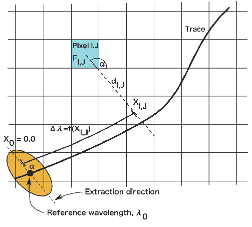
Figure 2: The geometry in a beam. \(\alpha\) is the orientation of an extended object. A single wavelength is assigned to each pixel within a beam. An extraction along an arbitrary direction \(\alpha\) with repect to the pixel grid is allowed. This optimizes the resolution of the final extracted spectrum.
The absence of slits and masks also dramatically enhances the probability that spectra of different sources overlap each other. Even at large distances along the dispersion direction, the different orders of two objects still can overlap and create confusion problems. aXe can mark and extract several dispersion orders per object to properly record the source confusion or contamination for every order of each object.
3.3. Apertures and Beams
The extraction process in aXe is done on the basis of so called BEAMs. Each beam comprises one dispersion order of one object. The collection of all beams (dispersion orders) of one object is called the APERTURE. The aperture is characterized by the aperture number, which is identical to the object number in the Input Object List. The beams are named with a single character. The alphabetical sequence (A, B, C, …) follows the sequence of beams defined in the Configuration File. Each beam is defined by the coordinates of the quadrangle which contains the pixels that are extracted together to form the spectrum of one dispersion order of an object.
The beams follow the spectral trace of the spectrum, which is defined in the Configuration File (see Configuration Files for a detailed description). While the length of a beam is set by the length of the corresponding dispersion order, its width is adapted to the extraction width set by the user.
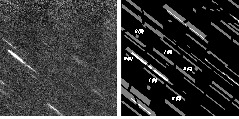
Figure 3: A grism image of the HUDF HRC Parallels Program (left panel) and the aXe-beams therein (right paenl). The numbers and characters give the spectra order and the beam label in aXe. The bright areas mark the overlap of several beams.
The left panel in figure 3 shows an HRC/G800L grism exposure reduced in the HUDF HRC Parallels Program (cleaned from cosmic-ray hits). In the right panel, some of the beams marked and extracted in aXe are indicated. The numbers give the spectral order, and the letters denote the correspondence with the beam in the configuration file. The bright areas mark regions where beams overlap and contaminate their spectra mutually. The different extraction angles for the objects result in different shapes of the marked regions. For each beam the description of the spectral trace and the wavelength assignment is set up and the spectral reduction is done independently.
3.4. Pixel Extraction Tables (PET)
An important step in the aXe reduction process is the generation of the so called Pixel Extraction Table (PET). A PET is a multi-extension fits-table which stores in each extension the complete spectral description of all pixels of one beam. figure 2 illustrates the geometry in a beam and shows various quantities stored in the PET. Important pixel information stored in the PET is:
the section point, defined as the point where the spectral trace intersects a line drawn through the centre of the pixel along the extraction direction
the distance to the section point \(d_{ij}\)
the trace distance \(X_{i,j}\) of the pixel (which is equal to the trace distance of the section point)
the wavelength attributed to the pixel (derived by inserting the trace distance into the dispersion function stored in the configuration file)
The PETs are read and manipulated by many aXe tasks. For example, a flat-field correction is applied to the pixel values stored in the PETs. Since flat-fielding is a wavelength dependent operation, the assignment of a wavelength to each pixel is required before the correction values, derived from a 3D flatfield cube are applied(see Flat Fields).
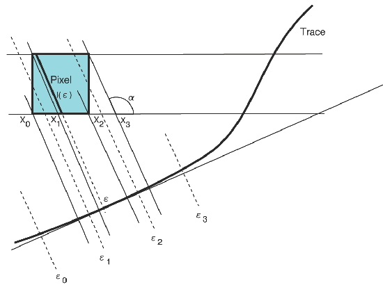
Figure 4: How a one-dimensional spectrum is created using information from the Pixel Extraction Table. Each pixel in the table is projected onto the trace into separate wavelength bins. The number count of each pixel is weighted by the fractional area of that pixel which falls onto a particular bin.
3.5. Generating 1D spectra
The geometry required to convert the contents of the PET to a set of one dimensional spectra stored in the Extracted Spectra File (SPC) (see extracted spectral formats) is shown in figure 4. The method accounts for the geometrical rotation of the square pixel with respect to the spectral trace and appropriately projects each pixel onto the trace. To do this a weighting function is used which is the fractional area of the pixel which, when projected onto the trace, falls within the bin points \(\epsilon_1\) and \(\epsilon_2\). The flux contained in each BEAM pixel is weighted by this weighting function as it is projected onto separate bins (\(\epsilon_0\) to \(\epsilon_1\), \(\epsilon_1\) to \(\epsilon_2\), and \(\epsilon_2\) to \(\epsilon_3\) in figure 2) along the spectral trace. The weight is computed by integrating over the length of the segments such as \(l(\epsilon)\) shown in figure 4. The length of these segments is nonzero from \(x_0\) to \(x_3\), reaches a maximum value of \(1/sin(\alpha)\), and rises and decreases linearly such that it can be described by:
Integration over this function \(l(x)\) to compute \(w(\epsilon_0,\epsilon_1), w(\epsilon_1,\epsilon_2)\), and \(w(\epsilon_2,\epsilon_3)\) is trivial once \(x_0,...,x_3\) have been computed, which are derived from simple trigonometry.

Figure 5: Left panel (a): The master sky for the HRC. The holder for the coronograph results int he ‘arm’ with low sensistivity at the top. Right panel (b): Background estimate for the grism image show in figure 3 with the object regions masked.
Once the one dimensional spectra have been generated, the final step of flux calibrating can be performed by applying a known sensitivity curve for the observing mode which was used. The output product of the aXe extraction process is a FITS binary table containing the set of extracted and calibrated spectra (see extracted spectral formats).
3.6. Sky Background
aXe has two different strategies for removal of the sky background from the spectra.
The first strategy is to perform a global subtraction of a scaled
master-sky frame from each input spectrum image at the beginning of
the reduction process. This removes the background signature from the
images, so that the remaining signal can be assumed to originate from
the sources only and is extracted without further background correction
in the aXe reduction. To enable global background subtraction in hstaxe,
set the backgr argument in the axeprep step to True, for example:
axetasks.axeprep(inlist="aXe.lis",
                 configs="G141.F140W.V4.31.conf",
                 backgr=True,
                 norm=False,
                 mfwhm=3.0)
The second strategy is to make a local estimate of the sky background
for each BEAM by interpolating between the adjacent pixels on either
side of the BEAM. In this case, an individual sky estimate is made for
every BEAM in each science image. Counter-intuitively, if you wish to
do local subtraction without doing a global subtraction first, you must
set backgr to False in the axeprep step:
axetasks.axeprep(inlist="aXe.lis",
                 configs="G141.F140W.V4.31.conf",
                 backgr=False,
                 norm=False,
                 mfwhm=3.0)
The strategy of estimating a local sky background can also be applied
after a global sky background subtraction for very difficult cases or
instruments (e.g. NICMOS G141 data, see [FREUDLING] ). In either case (with
or without previous global sky background subtraction), the local background
subtraction is used by setting back=True and specifying a value for
backfwhm, np, and interp in the axetasks.axecore step, for
example:
axetasks.axecore('aXe.lis',
                 "G141.F140W.V4.31.conf",
                 np=5,
                 interp=0,
                 back=True,
                 backfwhm=4.0,
                 [additional keyword arguments])
For additional information about these parameters, see Parameters and BACKEST. More information about local and global background subtraction is also given below.
In addition to global and local background subtraction, you can choose to
not perform any sky background subtraction at all by setting backgr=False
in the axeprep step and back=False in the axecore step.
3.6.1. Global Background Subtraction
The homogeneous background of HST grism exposures makes the global background subtraction from the pipeline processed science images (i.e. _flt.fits files) feasible. Master sky images for both ACS (WFC and HRC) and WFC3 are available from the instrument web pages at http://www.stsci.edu/hst/wfc3/analysis/grism_obs/wfc3-grism-resources.html
All master sky images were created by combining many grism images from different science programs. The object signatures on the science images were removed using several techniques, including a two step median combination, to derive a high signal-to-noise image of the sky background. figure 5 shows the ACS/HRC master sky image.
Scaling and subtraction of the master sky is done with the aXe task axeprep (see figure 3). Before scaling the master sky to the level of each science frame, the object spectra are masked out on both the science and the master sky image.
When reducing a dataset consisting of many individual exposures, it may be desirable to check the sky subtraction by co-adding all the sky-subtracted grism images (e.g., with the Astrodrizzle task). The co-added image also provides a way to quickly assess the quality of the background subtraction. Any deviations from zero in the mean background level of the combined image will also affect the spectra derived withthe aXe reduction.
3.6.2. Local Background Subtraction
The second option for handling the sky background is to make a local estimate of the background for each object. In this case, aXe creates an individual background image for each object on the spectrum image. On the background image the pixel values at the positions of the object beams are derived by interpolating in each column between the pixel values on both sides of the beam. The number of pixels used in the interpolation as well as the degree of the interpolating polynomial can be chosen by the user. figure 5 shows the background image corresponding to the grism image displayed in figure 3.
The background images are then processed in much the same way as the science images, resulting in a Background Pixel Extraction Table (BPET) for all BEAMs in a grism image. Thus, every PET has its corresponding BPET, derived from the background image, with the spectral information of the identical objects and beams in it. Finally, the BPET is subtracted from the PET and the background subtracted spectra are extracted.
3.7. Contamination
In conventional spectroscopy an overlay of spectra from different sources can occur only if two or more objects fall within the aperture defined by a slit or mask element. However in slitless spectroscopy there is no spatial filtering of sources. This allows both overlap of spectra from near neighbours in the cross dispersion direction as well as from more distant sources in the dispersion direction. For this reason spectral overlap or contamination is an ubiquitous issue for slitless spectroscopy, which must be explicitly taken into account in the data reduction.
3.7.1. Geometrical contamination
In geometrical contamination the areas covered by the different orders of all objects are recorded on a so-called contamination image. figure 3 and figure 6 show the contamination image for data taken in the Hubble Ultra Deep Field with the HRC and WFC, respectively. In both figures the regions marked black are covered by no spectrum at all, the white or red areas show regions which are covered by several (up to 15 in figure 6 overlapping spectra, which contaminate each other.
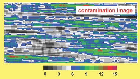
Figure 6: The contamination image compiled for data taken in the Hubble Ultra Deep Field The difference colours give the number of spectral orders which contaminate each other.
The information on the number of contaminating sources in figure 6 is stored in the object PET and fully propagated in the 1D extraction of the individual object spectra. As a final result each spectral element is accompanied by a flag which indicates whether its input pixels were also part of other object spectra. The regions of 1D spectra where the contamination flag is set must be used with care, since neighbouring sources also contribute to the extracted flux.
This contamination scheme is fast and very efficient in identifying problematic regions in the individual object spectra, however there is no information on the severity of the contamination.
The quantitative contamination introduced below assesses the contamination from neighbouring sources and helps to decide whether the contaminated spectrum might still be suitable for further scientific analysis.
3.7.2. Quantitative contamination
The quantitative contamination gives, for each spectral element, an estimate on the contaminating flux from all other sources. Based on this quantitative contamination estimation, the user has a better tool to decide which data points can be trusted.
The basis of the quantitative contamination estimation is a model which estimates the dispersed contribution of every object to the grism image. The contributions of the individual objects are then coadded to a 2D contamination image, which is a quantitative model of the examined grism image. In the 1D extraction of the individual object spectra, the model contribution of the object itself is subtracted (to avoid self-contamination), and then the data from the modelled grism image is processed in parallel with the data from the real grism image.
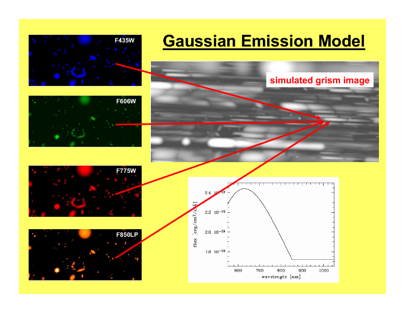
Figure 7: The Gaussian emission model for ACS/WFC: photometric information in four filters show on the left is emplyed to compute the model grism image(right). The object morphologies are approximated by 2D Gaussians. The arrows connect the direct image positions of one object to its first order grism spectrum. The photometric values are transformed to flux and interpolated as shown on the lower right side.
As a result two spectra for every object are derived: one extracted from the real grism image; and a second one extracted from the modelled grism image. Since the model contribution of the object itself was excluded in the extraction of the latter spectrum, this spectrum is a quantitative estimate of the contamination from all other sources to the object spectrum in question. The accuracy of the contamination spectrum is set by the accuracy of the emission model which is needed as an input to compute the modelled grism image.
Two different emission models have been implemented, called the Gaussian Emission Model and the Fluxcube Model
The Gaussian Emission Model
In the Gaussian emission model, the object morphologies are approximated by Gaussians with widths taken from the Input Object List. The Input Object List must also contain photometric information, which is provided by the total AB-magnitude in at least one filter passband or wavelength. In this mode the column name of the magnitude columns must indicate the wavelength with a simple format (such as MAG_F850LP for an AB-magnitude determined at 850nm, see Chapt. [SEX] for details on the column names). With a proper name for the magnitude column, the Input Object List, which is required to run aXe, contains all the data to compute the contamination with the Gaussian emission model.
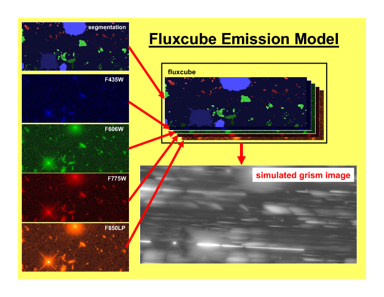
Figure 8: The Fluxcube emission model for ACS/WFC: reali images in four filters (left) are converted to flux images and combined with the segmentation image to a fluxcube file (upper right). The model grism image (lower right) is computed using the data in the fluxcube.
figure 7 displays on the left side the ACS/WFC direct images in the four observed filters as seen in the Gaussian emission model, which means all objects have Gaussian shapes. The upper right panel of figure 7 shows the modelled ACS/WFC/G800L grism image computed from the morphological and photometric information. The arrows point from the direct image positions of one object to the position of its first order spectrum in the modelled grism image. In order to compute the contribution of this object to the grism image, the four photometric values (AB-magnitudes at \(435\), \(606\), \(775\) and \(850\)nm) were transformed to flux and then interpolated with a cubic spline as shown in the lower right panel of figure 7. Outside the range of the photometric data a constant extrapolation of the last available data point is used.
The images in figure 7 cover the same area as the contamination image in figure 6. The direct images in figure 7 were only created for illustration purposes. In real aXe runs, each filter is just represented by a column in the Input Object List which gives the total AB-magnitude of the objects.
The Fluxcube Model
In the Fluxcube emission model both the object morphologies as well as the spectral information are taken from the fluxcube file associated with every grism image. A fluxcube file is a multi-dimensional fits image with one or several flux images taken at different wavelengths as extensions. The basis of the flux images are normal 2D images in \([counts/sec]\), which must be transformed to flux in \([erg/cm^2/s/\AA]\) using the appropriate zeropoints. All extensions of the fluxcube image must cover the same area as the corresponding grism image.
The flux extensions in the fluxcube provide sufficient information to compute a model grism image. In the determination of the quantitative contamination however it is essential to derive the individual contribution of each object to the modelled grism image. This addition is necessary to be able to subtract the self contamination and to isolate the contamination from other sources for each individual object.
For this reason the first extension of a fluxcube image must contain the so called “Segmentation Image”. In the segmentation image each pixel value is the (integer) number of the object to which the pixel is attributed. The SExtractor software provides the possibility to create a segmentation image (parameter setting: CHECKIMAGE_TYPE SEGMENTATION) as an additional output product of the source extraction.
The fluxcube files necessarily follow a rather complicated file format. To support the user in the creation of fluxcube files an aXe task has been implemented. The task fcubeprep works in a standard scenario with a drizzled grism image, one or several drizzled direct images and a segmentation image as input.
As an illustration of the Fluxcube model for ACS/WFC, figure 8 shows on the left side the segmentation image and the filter images used to create the fluxcube. The lower right part of figure 8 displays the modelled ACS/WFC/G800L grism image derived by the fluxcube emission model. All images in figure 8 cover the identical area of figure 7 and figure 6 in the HUDF.
More details on quantitative comtamination are given in and .
3.8. Drizzling of PETs
[drizzlingPETs] The aXe reduction scheme described up to now produces one spectrum for each individual beam in each science image. However, datasets, such as those obtained with ACS, often consist of several images with small position shifts (dithers) between them. The direct approach of co-adding the 1D spectra extracted from each image to form a combined, deep spectrum has several disadvantages:
The data is (non-linearly) rebinned twice, once when extracting the spectrum from the image and again when combining the individual 1D spectra;
A complex weighting scheme is required to flag cosmic ray affected and bad pixels;
Low level information on the cross dispersion profile is lost when many 1D extracted spectra are combined to a deep spectrum.
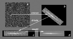
Figure 9: Drizzling in aXe: The object marked in panel (a) is extracted as a stamp image (b). The stamp image is drizzled to an image with constant dispersion and constant pixel scale in cross dispersion direction (c). The deep 2D drizzled image (d) is then used to extract the 1D spectrum.
To circumvent these drawbacks, there is a more advanced reduction scheme available, whereby all the individual 2D spectra of an object are coadded to a single deep 2D spectrum. The final, deep 1D spectrum is then extracted from this combined 2D spectral image. The combination of the individual 2D spectra is done with the Drizzle software, Fruchter & Hook (2002), which is available in the STSDAS package within IRAF.
The advantages of this technique as applied to slitless spectra can be summarised as follows:
Regridding to a uniform wavelength scale and a cross-dispersion direction orthogonal to the dispersion direction is achieved in a single step;
Weighting of different exposure times per pixel and cosmic-ray affected pixels are correctly handled;
There is only one linear rebinning step to produce a 2D spectrum;
The combined 2D spectra can be viewed to detect any problems.
These advantages come at the expense of a greater complexity of the reduction and significantly longer processing time. Also, the aXe drizzle reduction currently supports only first-order spectra.
The drizzling within aXe is fully embedded in the aXe reduction flow and uses data products and tasks created and used in the non-drizzling part of aXe. The input for the drizzle combination consists of flatfielded and wavelength calibrated PETs extracted for each science image, which are converted to Drizzle PrePare files (DPP) using the drzprep task. Every first order beam in a PET is converted to a stamp image stored as an extension in a DPP. The drzprep task also computes the transformation coefficients which are required to drizzle the single stamp images of each object onto a single deep, combined 2D spectral image. These transformation coefficients are computed such that the combined drizzle image resembles an ideal long slit spectrum, with the dispersion direction parallel to the x-axis and cross-dispersion direction parallel to the y-axis. The wavelength scale and the pixel scale in the cross-dispersion direction can be set by the user with keyword settings in the aXe Configuration File.
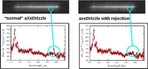
Figure 10: The comparison of a 2D drizzled image (WFC3/G141) produced with the “normal” aXedrizzle (left column) and the new aX3drizzle that can reject deviant pixels (right column). Hot or cosmic ray affected pixels without a correct flag in the data quality array are detected and masked out in the new aXedrizzle.
To finally extract the 1D spectrum from the deep 2D spectral image, aXe uses an (automatically created) adapted configuration file that takes into account the modified spectrum of the drizzled images (i.e. orthogonal wavelength and cross-dispersion and the \(A/pixel\) and \(arcsec/pixel\) scales).
A detailed discussion of the drizzling used in aXe is given in [KUMMEL4].
figure 9 illustrates the aXedrizzle process for one object. Panel a shows one individual grism image with an object marked. Panel b displays the stamp image for this object out of the grism image. Panel c shows the derived drizzled grism stamp image, and the final coadded 2D spectrum for this object is given in panel d. Panel d shows an image combined from 112 PETs with a total exposure time of 124 ksec. In both panels b and c, the holes resulting from the discarded cosmic ray-flagged pixels in this individual exposure are clearly visible.
For aXe version 2.1 we have extended aXedrizzle, and the new version offers to detect pixels with deviating values such as MultiDrizzle [KOEKEMOER] does in direct imaging. As is shown in figure 10, the new aXedrizzle is able to detect and mask out deviant pixels (right panels), thus reducing the risk to produce an emission line which is an artifact (left panels).
The new aXedrizzle can only be applied if the sky background has been subtracted off via global background subtraction (see Global Background Subtraction). This new method of combining the 2D grism stamp images has been developed on the basis of and for WFC3 G102 and G141 data. In principle, the new aXedrizzle could also be applied to ACS G800L data, however there exist other methods to reliably detect cosmic rays in these modes (see MultiDrizzle). The new aXedrizzle has certainly the potential of delivering better and cleaner spectra, as can be seen in figure 10. But if the alignment of the images has not been done properly, the new aXedrizzle can massively mask out good pixels and thus damage the resulting spectra. The results of the aXedrizzle with pixel rejection (task axedrizzle with driz_separate=YES, see AXEDRIZZLE) should only be taken as valid after a carefully comparison with the spectra from the basic aXedrizzle process (task axedrizzle with driz_separate=NO, see AXEDRIZZLE).
3.9. Optimal weighting
The use of unequal weights in the 1D extraction of spectral data can enhance the signal-to-noise ratio of the extracted spectra. The improvement is achieved by attributing lower weights to pixels which, due to the larger distance from the spectral trace, contain only a small fraction of the object flux. The optimal weighting technique was originally introduced in [HORNE], and the basic equation of the spectral extraction using optimal weights is (see [RODRIGUEZ] ):
The variables are:
\(\lambda\): the coordinate in the spectral direction
\(f(x, \lambda)\): the data value at pixel \((x,\lambda)\)
\(b(x, \lambda)\): the background value at pixel \((x,\lambda)\)
\(\sigma(x, \lambda)\): the noise value at pixel \((x,\lambda)\)
\(p(x, \lambda)\): the extraction profile at pixel \((x,\lambda)\)
\(f(\lambda)\): the extracted data value at \(\lambda\)
In the original descriptions of optimal weighting, the extraction profile \(p(x, \lambda)\) is computed from the object spectrum itself by e.g. averaging the pixel values in wavelength direction. In [HORNE] optimal weighting (or optimal extraction, as named there) is even an iterative procedure which, starting from a normal extraction procedure using equal weights, produces improved results for sky background, extraction profile and, of course, the extracted spectrum.
In ACS slitless spectroscopy such an approach is not viable since
an iterative approach on the sometimes hundreds or even thousands of spectra on a slitless image would require too much computing time;
the signal-to-noise ratio of the sources is often too low to determine an individual extraction profile;
the contamination phenomenon does not permit an automatic and reliable generation of extraction profiles for all sources.
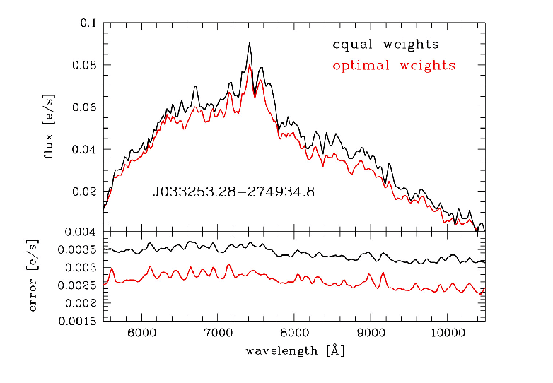
Figure 11: The comparison for an aXe extraction with (red) and without (black) optimal weights. The upper panel compares the object flux, the lower panel shows the associated errors.
To compute extraction profiles for all sources, the optimal weighting as implemented in aXe uses the 2D models for the dispersed objects, which were introduced in Quantitative contamination as the basis of quantitative contamination. The source-specific models computed there deliver a perfect basis to calculate the quantity \(p(x, \lambda)\) in equation (2).
The beam models are also used as an input to calculate the pixel errors \(\sigma(x, \lambda)\) according to the typical CCD noise model
with \(mod(x, \lambda)\) and \(rdnoise\) the beam model value at pixel \((x,\lambda)\) and the CCD readout noise, respectively. Computing the quantitative contamination estimate with either the Gaussian or the Fluxcube emission model is therefore a precondition to optimal weighting.
In all extraction modes (from individual grism images or from the
combined 2D drizzled grism images) aXe delivers optimal weighted spectra
as an optional addition to the usual, equally weighted ones.:num:figure #extr-comp
shows a comparison between two spectra extracted
from the same data using equal and optimal weights. Results from both
observed as well as simulated data indicate that optimal weigthing in
aXe improves the signal-to-noise ratio by a small, but significant
amount as expected according to [HORNE] and [ROBERTSON].
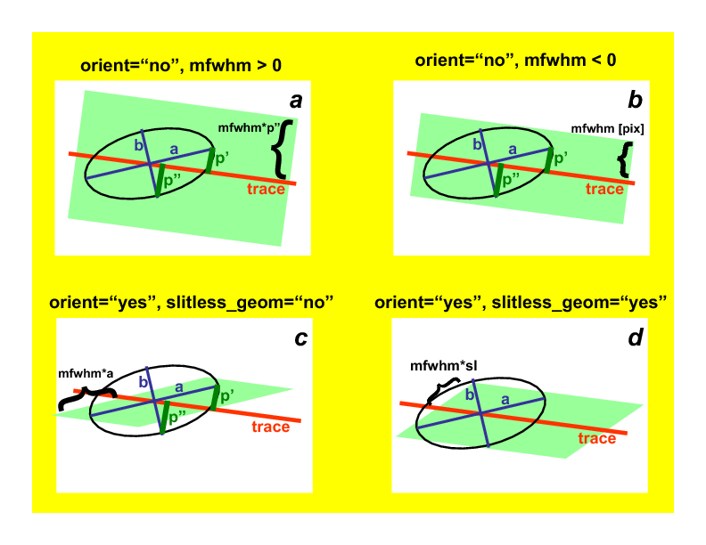
Figure 12: The four different methods to extract 1D spectra: (a) perpendicular to the trace, with an object specific extraction width \(mfwhm * M A X(p', p'')\) and \(p'\) and \(p''\) the projection of the major and minor half axis width onto the extraction direction, respectively; (b) perpendicular to the trace, with a fixed extraction width \(mfwhm\) for all objects; (c) along the direction of the objects major have axis with extraction width of \(mfwhm * a\) (a= major axis width); (d) a virtual slit with the length sl, widht sw and orientation so as computed from the morphological object parameters \((a,b,\sigma)\) to extract with the width \(mfwhm * sl\) along so.
3.10. Extraction parameters in aXe
aXe offers a large range of possibilities to specify the extraction width and extraction direction for the individual objects. Before running aXe, the user has to decide in which way the 1D spectra should be extracted from the grism images.
3.10.1. Fixed extraction direction or variable extraction direction
With a fixed extraction direction the lines of constant wavelength and therefore the extraction direction form the angle \(90^\circ\) with the trace in all beams of all objects.
With variable extraction, the line of constant wavelength follows for every object a specific, marked direction. The major axis angle in the column THETA_IMAGE of the Input Object List is used in this mode to define the line of constant wavelength or extraction direction for every object individually. aXe mimics with the variable extraction direction individually oriented slits for all objects. This can help to maintain the instrumental resolution for small, extended objects. However for small angles between the trace and the extraction direction the finite instrumental resolution limits any improvements due to the variable extraction direction, and in addition the extraction becomes numerically unstable. aXe can switch (with the parameter SLITLESS_GEOM=YES, see below) the extraction direction from the major axis angle to a different angle which optimizes the resolution of the extracted spectra (see [KUMMEL2], [FREUDLING]).
Note
The optimal choice of extraction strategy depends very much on the scientific goals ans the morephology of the observed sources. For stellar sources a fixed extraction direction together with a fixed extraction width is cer- tainly highly recommended. Deep survey type observations definitely need a variable extraction width, since the object sizes usually span a large range which can not be met with a fixed extraction width. In this case the re- sults would also benefit from a variable extraction direction to get the best possible spectral resolution. Also in typical survey scenarios the morphological description of stellar objects and faint objects close to the detection limit rather reflects the statistical or systematic measurement errors than the true intrinsic object properties. To compensate these doubtful mesurements of the quantities A IMAGE, B IMAGE and THETA IMAGE, aXe applies, with the parameters op- timized for surveys, a default extraction with an extraction direction per- pendicular to the trace angle and a fixed object size to all objects smaller than a threshold given in the configuration file. Setting this threshold to the typical size of point-like objects assures a proper extraction for stellar objects and marginally resolved faint sources.
Warning
The parameter combination ORIENT=yes and SLITLESS_GEOM=NO might be resonable in isolated cases, and it’s use is not prohibited. However aXe delivers a warning in the case that the angle between the extraction direction and the object trace is very small (\(<1^\circ\)). This warning must be seriously taken into account, since a core dump may result during later stages of the aXe reduction
3.10.2. Fixed extraction width or object specific extraction width
Similar to the choice of extraction direction, aXe offers both a fixed and a variable extraction width. The fixed extraction width remains constant for all objects.
The variable extraction width is determined for each object individually to a scaled value \(extrfwhm\) of the object extent in the extraction direction.
The main parameters to specify extraction width and extraction direction are extrfwhm (or \(mfwhm\) in figure 12, orient and slitless_geom in the task axecore. figure 12 illustrates how those parameters can be used to extract the flux of an object in various ways:
in figure 12 a, the flag orient=NO indicates a fixed extraction direction of \(90^\circ\) with respect to the trace direction. A value mfwhm > 0 specifies a variable extraction width, which in the case orient=NO is \(width = MAX(p', p'') * mfwhm\) pixels on either side of the trace (hence \(2*width\) in total). Here \(p'\) and \(p''\) are the projection of the major and the minor axis width onto the extraction direction.
in figure 12 b, the flag orient=NO indicates a fixed extraction direction of \(90^\circ\) with respect to the trace direction. A value mfwhm < 0 specifies a fixed extraction of \(width = mfwhm\) pixels on each side of the trace (hence \(2*mfwhm\)pix in total).
in figure 12 c, the flag orient=YES indicates a variable extraction direction. Since slitless_geom=NO the extraction direction must follow the direction of the major axis \(a\). The extraction width is variable with \(width = mfwhm * a\) pixels on either side of the trace.
in figure 12 d, with the flag slitless_geom=YES an individual virtual slit with the slit length sl, the slit width sw and the orientation so is defined from the major axis size A_IMAGE, the minor axis size B_IMAGE and the major axis angle THETA_IMAGE given in the Input Object List. Appendix A gives the equations for computing the virtual slit parameters. The shape of the virtual slit optimizes the spectral resolution for the extracted spectra and avoids angles too close with the trace direction (see and for details). The extraction width is then the object specific width \(width = mfwhm * sl\) along the direction so.
3.11. Flux conversion
The flux conversion is done using sensitivity curves which had been derived through dedicated observations of flux standard stars ([KUNTSCHNER],[LARSON1]_,[LARSON2]_). In extended objects, however, the spectral resolution is degraded by the object size in the dispersion direction. aXe can take into account (parameter adj_sens=YES in the tasks axecore, axedrizzle, pet2spc) the degraded spectral resolution of extended sources by smoothing the point source sensitivity function. Based on the approximation of Gaussian object shapes, aXe uses a Gaussian smoothing kernel with the width
with \(sw_i\) the width of the virtual slit of object \(i\) (see Appendix A), the dispersion \(r\), the point source object width \(p\) and the correction factor \(f\), which is empirically determined for the various slitless modes. The adjusted flux conversion has been developed for and applied in the various data reduction projects within the Hubble Legacy Archive (HLA) program [FREUDLING].
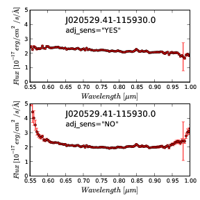
Figure 13: An ACS.WFC G800L slitless spectrum of an extended object reduced with (upper panel) and without (lower panel) adjusting the sensitivity curve in the flux conversion. The ‘wings’ at both wavelength ends in the lower panel are a clear sign of the decreased resolution due to the object extent.
figure 13 shows the effect of the sensitivity adjustment for an extracted ACS/WFC spectrum. The lower panel shows a strong upturn at both wavelength ends due to the degraded resolution. Smoothing the sensitivity function using the appropriate Gaussian kernel suppresses this effect (upper panel).
3.12. aXe Visualization
A deep ACS/WFC grism image can contain detectable spectra of hundreds to thousands of objects, and visual checking of each spectrum is very tedious. A quick-look facility is highly desirable in order to find interesting objects (e.g. high redshift galaxies, SN, etc) which can be highlighted for further study or interactive spectrum extraction. For this reason aXe2web was developed, a tool which produces browsable web pages for fast and discerning examination of many hundreds of spectra.
Since aXe2web requires specific python modules, it cannot be included in the STSDAS software package. It is therefore distributed via the aXe webpage at in the aXe2html package.
aXe2web uses a standard aXe input catalogue and the aXe output files to produce an html summary containing a variety of information for each spectrum. This includes a reference number, magnitude in the magnitude system of the direct object, the X and Y position of the direct object, its Right Ascension and Declination, a cut-out image showing the direct object, the spectrum stamp image showing the 2D spectrum, a 1D extracted spectrum in counts and the same in flux units.
The user can set various keywords to influence the html output. For example, it is possible to sort the objects with respect to an object property such as magnitude or Right Ascension.
In order to facilitate the navigation within a data set, an overview and an index page accompany the object pages. The overview page contains for each object the basic information sequence number, reference number, X,Y,RA,Dec and magnitude. The index page includes a table with the ordered reference number of all objects. Direct links, from both the overview page and the index page, point to the corresponding locations of the objects in the object pages.
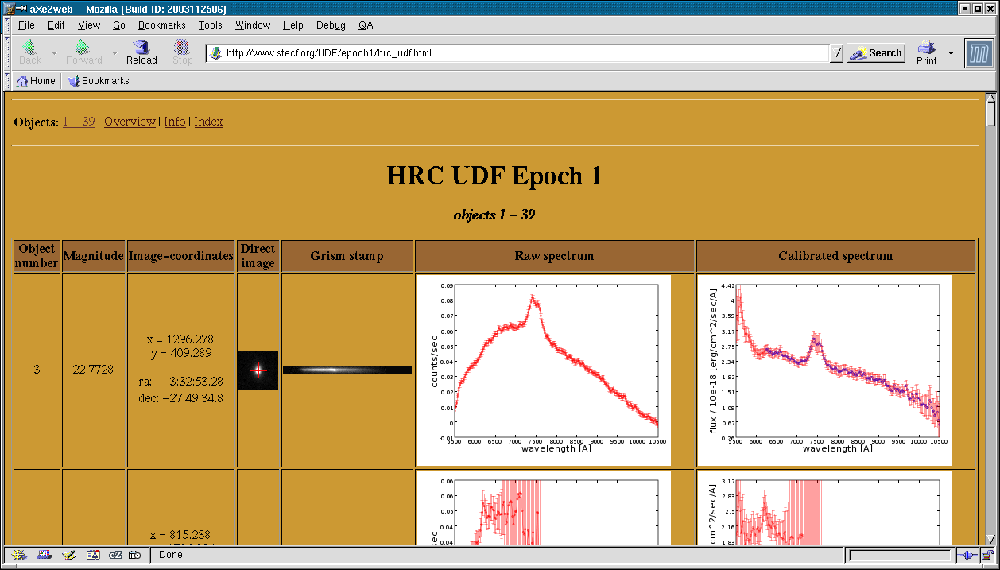
Figure 14: Part of a webpage created by aXe2web. The coadded 2D spectrum of the object shown here is displayed in figure 9.
figure 14 is a screenshot taken from Epoch 1 data of the HUDF HRC Parallels survey and shows the line covering the object whose coadded 2D spectrum is shown in Fig. [drizzle]d. The web pages created by aXe2web are located at the preview web pages: http://archive.stsci.edu/prepds/udf/
3.13. Acknowledgement
In publications, please refer to aXe as: Sosey, M., Pirzkal N., Lee, J. 2013