5. Using hstaxe
This chapter gives a step-by-step approach on how an aXe reduction on a given data set is performed. A short introduction to the input data is followed by an explanation of the few preparatory steps that are necessary to generate all input files. Then the different methods to produce the final, calibrated 1D spectra are shown and discussed. Both the sequence of commands within PyRAF as well as small example scripts are given for all reduction branches.
5.1. The input data
The input data consist of four direct images and eight grism images. All images were taken with the High Resolution Camera of the ACS. The direct images taken with the F555W filter are
j8m81cd9q_flt.fits
j8m824toq_flt.fits
j8m84aqkq_flt.fits
j8m851tmq_flt.fits
The dispersed images observed with the G800L grism are:
j8m820leq_flt.fits
j8m820llq_flt.fits
j8m820lrq_flt.fits
j8m820m4q_flt.fits
j8m822q0q_flt.fits
j8m822q4q_flt.fits
j8m822qbq_flt.fits
j8m822qhq_flt.fits
The data set presented here is in the HST archive. It has been taken as part of the ACS/HRC Parallels program to the ACS Ultra Deep Field. Moreover these images are also part of the test data for grism observations.
Warning
Spectral extraction from MultiDrizzled grism/prism images: While MultiDrizzle can combine slitless grism/prism images, no wavelength sensative flatfield is applied to the images (see Flat field). Moreover, the field dependence of the grism/prism spectra and the field dependent wavelength calibration are not taken into account in the combination process. It is therefore not recommended to extract the spectra directly from the Multidrizzle combined images. The images are however very useful for field examination.
5.2. Preparing the extraction
This reduction step collects all necessary input files for the spectral extraction. In this process the external programs SExtractor [BERTIN] and Astrodrizzle (part of the drizzlepac package) are involved. For those programs outside of aXe we do not give a detailed discussion on their usage or the exact parameter settings, but rather a description of the purpose and what the program should deliver.
5.2.1. MultiDrizzle
The first step is to run MultiDrizzle on both the set of direct images and the set of grism/prism images. MultiDrizzle is an interface for performing all the tasks necessary for registering dithered HST images. The program automatically performs cosmic ray rejection, removes geometric distortions and performs the final image combination with drizzle.
The grism/prism image combination is done for two reasons:
the combined image gives a good impression on the quality of the data and the signal-to-noise level of the various object spectra
MultiDrizzle runs a cosmic ray detection algorithm, and the dq-extention of the flt-images is updated with the information on all cosmic rays detected in the MultiDrizzle run. Running MultiDrizzle is therefore a convenient way to perform a cosmic ray detection on the grism/prism images.
The combined direct image will be used to create a master catalogue with SExtractor. The master catalogue will then be projected back (see Preparing the Input Object Lists) to generate Input Object Lists for each image in the MultiDrizzle combination to be used in the aXe reduction. figure 1 shows an example of a combined direct image (left) and a combined grism image (right).
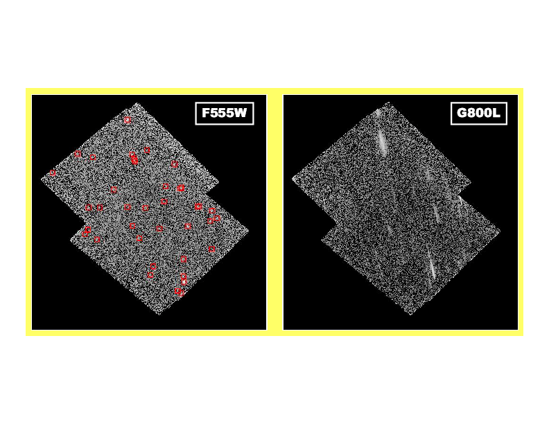
Figure 1: The MultiDrizzle combined direct image (left) and the corresponding grism image(right). Objects identified in SExtractor are marked with red boxes on the firect image.
It is also possible to use other programs to identify cosmic ray hits on the grism/prism images. Then the information on the cosmics must be transported into the dq-extension of the corresponding flt-image. aXe can exclude flagged pixels in the dq-extention from the reduction. In the dq-extention, cosmic ray affected pixels should be marked by adding the appropriate dq-flag 4096 (see ACS Data handbook) to the original dq value.
For grism images it is favourable (see Preparing the Input Object Lists) to combine the direct and the grism images such that the final, MultiDrizzled images have the same coordinate system. This means that each pixel \((x,y)\) represents the same position \((ra, dec)\) on the sky on both the combined direct as well as the combined grism image. The user can control this by e.g. specifying the identical center position and image size in the MultiDrizzle runs. The images in figure 1 fulfill this condition.
5.2.2. Master catalogue
The next step then is to create the master catalogue by running SExtractor on the combined direct image. Care should be taken when choosing the SExtractor parameters. Objects which are not in the master catalogue will later not be extracted from the grism images. Large numbers of fake objects or cosmics in the master catalogue on the other hand increase the computation time and simulate contributions to the contamination of real objects.
The master catalogue must contain all columns which are necessary for the spectral extraction with aXe (see the format description). The first few lines of the master catalogue f555w_drz.cat extracted from the direct image in figure 1 are:
#   1 NUMBER          Running object number
#   2 X_IMAGE         Object position along x                         [pixel]
#   3 Y_IMAGE         Object position along y                         [pixel]
#   4 X_WORLD         Barycenter position along world x axis          [deg]
#   5 Y_WORLD         Barycenter position along world y axis          [deg]
#   6 A_IMAGE         Profile RMS along major axis                    [pixel]
#   7 B_IMAGE         Profile RMS along minor axis                    [pixel]
#   8 THETA_IMAGE     Position angle (CCW/x)                          [deg]
#   9 A_WORLD         Profile RMS along major axis (world units)      [deg]
#  10 B_WORLD         Profile RMS along minor axis (world units)      [deg]
#  11 THETA_WORLD     Position angle (CCW/world-x)                    [deg]
#  12 MAG_F555W       Kron-like elliptical aperture magnitude         [mag]
 1 2116.6 815.9 5.322e+01 -2.781e+01 14.669 3.407 -79.3 1.0e-04 2.5e-05 -45.4 23.0
 2 1463.7 740.1 5.322e+01 -2.781e+01  1.981 1.355 -84.5 1.3e-05 9.4e-06 -42.8 26.1
 3  850.8 752.1 5.321e+01 -2.782e+01  1.877 1.749  21.9 1.2e-05 1.2e-05  37.9 24.6
 4 1999.1 735.0 5.322e+01 -2.781e+01  0.952 0.465 -52.7 6.0e-06 4.1e-06 -67.4 28.0
 5  760.5 761.5 5.321e+01 -2.782e+01  2.268 1.375 -54.4 1.4e-05 1.0e-05 -65.2 26.2
 6  969.0 826.9 5.322e+01 -2.782e+01  3.863 1.672  37.6 2.4e-05 1.5e-05  22.2 25.0
 7  781.3 831.3 5.322e+01 -2.782e+01  4.455 2.084 -58.9 2.9e-05 1.7e-05 -59.9 25.5
 8  976.5 826.2 5.322e+01 -2.782e+01  2.410 0.839 -86.7 1.6e-05 5.7e-06 -41.6 26.3
 9 1231.5 836.1 5.322e+01 -2.781e+01  2.522 1.177 -65.9 1.6e-05 9.3e-06 -53.8 25.9
10  981.5 834.9 5.322e+01 -2.782e+01  2.467 1.151  28.3 1.6e-05 9.5e-06  32.7 26.6
In the master catalogue the original column name MAG_AUTO was changed to MAG_F555W, a column name format which indicates the filter wavelength (\(\lambda=555.0\)nm, see Chapt. ). This format allows a quantitative contamination estimate with the Gaussian emission model and the computation of optimal weights.
5.2.3. Preparing the Input Object Lists
Following user requests we have developed and introduced with aXe-1.5 the task iolprep (see Chapt. [IOLP]), a program to automatically generate Input Object Lists in a standard scenario such as described here.
The task iolprep searches in the header of a MultiDrizzle-combined image for the names and drizzle parameters of all input images. For each input image, the pixel coordinates \((x_{comb},y_{comb})\) of all objects in the master catalogue, which is associated with the MultiDrizzle-combined image, are projected out into the coordinate system of the input image to derive the pixel coordinates \((x_{input,i},y_{input,i})\) therein. For each input image an Input Object List is generated which comprises all objects which fall on the area covered by the input image. For the projections of the object positions, this aXe task uses the STSDAS task tran.
There are two general strategies to apply iolprep:
1. Creating IOL’s for direct images
[case:sub:1] It is always (for grism and prism data) possible to apply
iolprep with the direct image as the MultiDrizzle-combined image and the
master catalogue derived from it. On a data set as described in
Chapt. [indata], the following IOL’s would be produced:
j8m81cd9q_flt_1.cat, j8m824toq_flt_1.cat,
j8m84aqkq_flt_1.cat, j8m851tmq_flt_1.cat.
As the file names suggest, the IOL’s refer to the direct images, and during the spectral extraction a direct image must be given for every grism image (see Chapt. [inlist]).
2. Creating IOL’s for grism images
[case:sub:2] If in the case of grism data MultiDrizzle was run such
that the combined direct and grism image have the same coordinate system
(see Chapt. [MultiDrizzle]), the object positions in the master
catalogue are also valid for the combined grism image. It is then
possible to apply iolprep with the grism image as the
MultiDrizzle-combined image. In this case the IOL’s refer to the input
grism images and would be named:
j8m820leq_flt_1.cat, j8m820llq_flt_1.cat,
j8m820lrq_flt_1.cat, j8m820m4q_flt_1.cat,
j8m822q0q_flt_1.cat, j8m822q4q_flt_1.cat,
j8m822qbq_flt_1.cat, j8m822qhq_flt_1.cat.
In this scenario the IOL’s refer directly to the grism images, as their file names indicate, and in the spectral extraction no direct image is needed.
The latter strategy has small advantages, such as it is easier to make the Input Image List (see below). It is possible to include objects in the Input Object List which have positions outside of the area covered by the corresponding direct image or grism image. In the case that the spectrum of the object falls partly on the grism image, but its reference point is outside, the spectrum covered by the grism image can still be reduced and contribute to the coadded spectrum of the object. Also higher orders of bright objects outside of the grism image can cause significant contamination on the grism images. Including them in the IOL means that their contamination is properly recorded and evaluated, even if no spectrum is extracted. The parameter dimension_info controls the effective area for the inclusion of objects in the task iolprep.
Depending on whether iolprep is run on the direct image f555w_drz.fits or the grism image g800l_drz.fits, the task is executed as:
-->iolprep mdrizzle_image='f555w_drz.fits' input_cat='f555w_drz.cat'
dimension_info=0,0,0,0
or alternatively:
-->iolprep mdrizzle_image='g800l_drz.fits' input_cat='f555w_drz.cat'
dimension_info=0,0,0,0
5.2.4. Preparing the fluxcube files
[fcubeprep] For grism images it is possible to apply the fluxcube emission model (see Chapt. [quantcont]) in the estimation of quantitative contamination. This requires the preparation of a fluxcube file for every grism image which is analyzed in aXe. For this purpose the task fcubeprep was developed.
Similar to iolprep, the task fcubeprep (see Chapt. [FPREP]) uses MultiDrizzled direct and grism images to build the fluxcube files. In addition, the SExtractor segmentation image which is associated to the master catalogue must also be provided. fcubeprep searches in the header of the MultiDrizzle-combined grism image for the names and drizzle parameters of all input grism images. Using the information on wavelength and zeropoints which are part of the input, the task transforms the direct images to flux units. Then the segmentation image and all direct flux images are projected into the coordinates of each input grism image to generate cutout images which match the area of the input grism images. For each input grism image, a fluxcube image is finally created from the corresponding segmentation and flux cutout images.
All images used in the input (MultiDrizzle-combined grism image, MultiDrizzle-combined direct images and segmentation images) must have been combined such that they have the same coordinate system. This means each pixel \((x,y)\) must represent the same position \((ra, dec)\) on the sky on all input images (see Chapt. [MultiDrizzle]).
In case there are several MultiDrizzle-combined direct images in different filters available, the user must prepare a file and give for each image the name, central wavelength and zero point separated by ’,’ in a row. Provided that in addition to the direct image f555w_drz.fits, there exists also the image f606w_drz.fits, this file (name dir_ims.lis) looks like:
f555w_drz.fits, 431.8, 25.157
f606w_drz.fits, 591.8, 26.655
Note that instead of the ’nominal’ values 555 and 606 the more accurate pivot wavelength values have been used for the ACS filters F555W and F606W. With the segmentation image f555w_seg.fits the task fcuberep is executed as:
--> fcubeprep grism_image='g800l_drz.fits' segm_image='f555w_seg.fits'
filter_info='dir_ims.lis' AB_zero='yes' dimension_info=0,0,0,0
The task creates the fluxcubes:
j8m820leq_flt_2.FLX.fits, j8m820llq_flt_2.FLX.fits,
j8m820lrq_flt_2.FLX.fits, j8m820m4q_flt_2.FLX.fits,
j8m822q0q_flt_2.FLX.fits, j8m822q4q_flt_2.FLX.fits,
j8m822qbq_flt_2.FLX.fits, j8m822qhq_flt_2.FLX.fits.
5.3. Extracting spectra
5.3.1. Reduction Strategy
[reduction strategy] Before actually preparing and performing the data reduction, the user must decide which data reduction strategy to follow.
The main decisions are whether aXedrizzle is used or not and whether the background subtraction is done globally with the master background or with a local background for each beam (see Chapt. [skyback] for a comparison of the two methods).
aXedrizzle is currently not supported for prism data. Global background subtraction requires a master background for the instrumental configuration with which the data were taken with. The available master background images are posted on the instrument pages ( http://www.stsci.edu/hst/acs/analysis/STECF and http://www.stsci.edu/hst/wfc3/analysis/grismobs/), and users are urged to check whether a master background is available for their data.
If possible, the recommended reduction strategy is to do a global background subtraction and to use aXedrizzle. For the typical survey type data, this is the best way to reduce ACS grism data (see e.g. the GRAPES data paper, Pirzkal et al., 2004) or WFC3 grism data. In case only individual spectra in crowded fields are to be reduced, the reduction with a background PET may have advantages.
Depending on the reduction strategy, different High Level aXe Tasks (see Fig. [figtasklist]) have to be applied to reduce the spectra. Table [taskseq] lists the tasks and the order in which to apply them for the various reduction strategies.
5.3.2. Input Image List
The Input Image List is consistently used as the parameter inlist in all High Level Tasks. The Input Image List defines the combinations of Input Object Lists, grism images and, if necessary, direct images used in the spectral extraction.
In case that the IOL’s refer directly to the grism images (see item 1. in Chapt. [case1]), the Input Image List axeprep.lis for the data presented here looks like:
j8m820leq_flt.fits j8m820leq_flt_1.cat 0.0
j8m820llq_flt.fits j8m820llq_flt_1.cat 0.0
j8m820lrq_flt.fits j8m820lrq_flt_1.cat 0.0
j8m820m4q_flt.fits j8m820m4q_flt_1.cat 0.0
j8m822q0q_flt.fits j8m822q0q_flt_1.cat 0.0
j8m822q4q_flt.fits j8m822q4q_flt_1.cat 0.0
j8m822qbq_flt.fits j8m822qbq_flt_1.cat 0.0
j8m822qhq_flt.fits j8m822qhq_flt_1.cat 0.0
If the IOL’s refer to direct images, (see item 2. in Chapt. [case1]), the Input Image List axeprep.lis for the data presented in here looks like:
j8m820leq_flt.fits j8m84aqkq_flt.cat j8m84aqkq_flt.fits  0.0
j8m820llq_flt.fits j8m81cd9q_flt.cat j8m81cd9q_flt.fits  0.0
j8m820lrq_flt.fits j8m81cd9q_flt.cat j8m81cd9q_flt.fits  0.0
j8m820m4q_flt.fits j8m84aqkq_flt.cat j8m84aqkq_flt.fits  0.0
j8m822q0q_flt.fits j8m851tmq_flt.cat j8m851tmq_flt.fits  0.0
j8m822q4q_flt.fits j8m824toq_flt.cat j8m824toq_flt.fits  0.0
j8m822qbq_flt.fits j8m824toq_flt.cat j8m824toq_flt.fits  0.0
j8m822qhq_flt.fits j8m851tmq_flt.cat j8m851tmq_flt.fits  0.0
Every grism image is paired with the direct image taken at the closest position on the sky to provide the best overlap between objects in the IOL and the area covered by the grism image. The dmag-values are all set to the default \(0.0\), and therefore could be neglected here.
The exact format of the Input Image List is extensively described in Chapt. [inlist]. All files are expected to be located in the directory indicated by the environment variable AXE_IMAGE_PATH (see Chapt. [Env Var]).
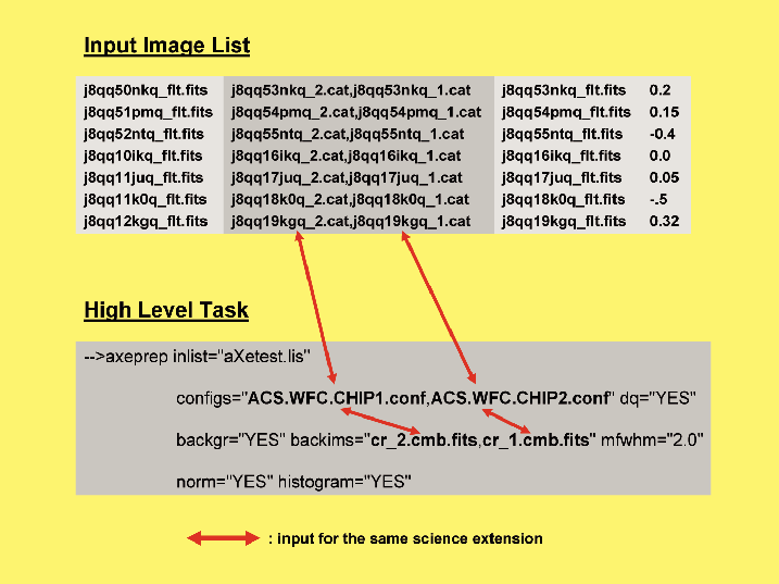
Figure 2: The input image list aXetest.lis and a high level aX3 task. The arrows connect input which refers to the identical science extension
5.3.3. The aXe Configuration Files
[Main Configuration File] The aXe configuration file describes the imprint of the spectrograph on the detector and contains essential parameters such as the desription of the spectral trace and the dispersion solution together with their variations over the Field of View.
Up-to-date configuration files and the calibration files for all spectral modes are posted on the instrument pages ( http://www.stsci.edu/hst/acs/analysis/STECF and http://www.stsci.edu/hst/wfc3/analysis/grismobs/). The appropriate configuration file for the data presented in this Chapter is given below. To save space the descriptions of the higher order beams are neglected.
INSTRUMENT ACS
CAMERA HRC

# Calibrations for ACS HRC for Cycle 11 onward; released June 2004
# based on calibration data taken during SMOV and Cycle 11.
# Revised (3rd order) flat field cube:
#   ACS.HRC.flat.cube.2.fits
#
# Revised 1st and 2nd order sensitivity
# New 0th order dispersion solution and sensitivity
# New -1st order dispersion solution and sensitivity
# March 2009 (MK): keywords 'POBJSIZE' 'SMFACTOR' with dummy values added

SCIENCE_EXT SCI ; Science extension
DQ_EXT DQ       ; DQ extension
ERRORS_EXT ERR  ; Error extension
FFNAME ACS.HRC.flat.cube.2.fits
DQMASK      16383

EXPTIME EXPTIME
RDNOISE 4.71
POBJSIZE 1.0
SMFACTOR 1.0

DRZRESOLA  24.0
DRZSCALE  0.028
DRZLAMB0  4785.0
DRZXINI   15.0
DRZROOT   aXedrizzle

# PSF variations for optimal extraction
PSFCOEFFS 8.20 -8.29e-02 4.01e-04 -9.47e-07 1.18e-09 -7.44e-13 1.87e-16
PSFRANGE 100.0 1100.0

# First order (BEAM A)
BEAMA 0 185
MMAG_EXTRACT_A 25
MMAG_MARK_A 27
# Trace description, 1st order
DYDX_ORDER_A 1
DYDX_A_0 0.0 0.0 0.0 0.0 0.0 0.0
DYDX_A_1 -0.796319 7.10246e-6 9.55948e-6
# X and Y Offsets
XOFF_A 0. 0. 0.
YOFF_A -1.78463 -0.000149007 0.000436432
# Dispersion solution, 2nd order
DISP_ORDER_A 2
DLDP_A_0 4783.55 0.00657371 -0.0126691
DLDP_A_1 23.5107 -0.000677401 0.00127958
DLDP_A_2 0.00170758 1.77847e-7 1.97777e-7
#
SENSITIVITY_A ACS.HRC.1st.sens.2.fits
Under normal circumstances the user can apply the aXe configuration files without any modifications. Only to speed up the computation time it might be convenient to modify some keywords (see Chapt. [timerequirements]). The location of the configuration and calibration files is the directory indicated by the environment variable AXE_CONFIG_PATH (see Chapt. [Env Var]).
The ACS Wide Field Camera and the WFC3 UVIS Camera contain two CCD chips, and the data is stored in two independent extensions of the fits file. The spectral reduction in aXe is done independently, using one configuration file for every science extension. In the ACS/WFC and WFC3/UVIS configuration files, the chip number is specified in the keywords “OPTKEY1” and “OPTVAL1”.
For technical reasons in both cameras the data of CCD chip No. 1 are stored in the second science extension version ( in PyRAF-fits notation), and the data of of CCD chip No. 2 is stored in the first science extension version ( in PyRAF-fits notation). Care must be taken to combine the correct files in the aXe input parameters, since the file names are often derived from these two counter-intuitive numbering schemes. While the file names of the configuration files follow the chip numbers (e.g. ACS.WFC.CHIP1.Cycle13.2.conf and ACS.WFC.CHIP2.Cycle13.2.conf are the configuration files for chip 1 and 2, respectively), the IOL’s created in iolprep follow the extension version number (the Input Object Lists j8m822qhq_flt_1.cat and j8m822qhq_flt_2.cat contain objects located on the fits image j8m822qhq_flt.fits[sci,1] and j8m822qhq_flt.fits[sci,2], respectively). Figure [inputext] and the note on page give further examples how to combine the input for ACS/WFC data in the various High Level Tasks.
5.3.4. Example reductions for the different scenarios
For the remainder of this section we present and describe sequences of High Level Tasks to reduce data according to the different strategies outlined in Chapt. [reduction strategy]. The High Level Tasks are listed with the correct syntax to be executed within an interactive PyRAF session.
aXedrizzle and Global Sky Subtraction
In this reduction scenario the background is subtracted using the mastersky HRC.back.fits . For each object the 2D spectra on the individual grism images are combined to a deep, 2D grism spectrum with aXedrizzle, then the 1D spectrum is extracted from the coadded 2D grism spectrum. The quantitative contamination with the fluxcube emission model is chosen. This assumes that the fluxcube files were created beforehand (see Chapt. [fcubeprep]).
As in all further examples, optimal extraction is selected in the parameters. In aXe the optimal extracted spectra are always delivered in addition to the normal, equally weighted results. There is no need to run aXe twice, the optimal extractions only entails but a small additional amount of computing time.
The sequence of commands interactively applied in PyRAF is:
-->axeprep inlist="axeprep.lis" configs="ACS.HRC.Cycle11.2.conf"
           backims="HRC.back.fits" backgr="YES" fwhm="2.0"
           norm="YES" histogram="YES"
-->axecore inlist="axeprep.lis" configs="ACS.HRC.Cycle11.2.conf"
           back="NO" extrfwhm=4.0 drzfwhm=3.0
           backfwhm=0.0 slitless_geom="YES" orient="YES" exclude="NO"
           lambda_mark=800.0 cont_model="fluxcube" model_scale=3.0
           inter_type="linear" lambda_psf=555.0 spectr="NO"
           weights="NO" sampling="drizzle"
-->drzprep inlist="axeprep.lis" configs="ACS.HRC.Cycle11.2.conf"
           opt_extr="YES" back="NO"
-->axedrizzle inlist="axeprep.lis" configs="ACS.HRC.Cycle11.2.conf"
              infwhm=4.0 outfwhm=3.0 back="NO" makespc="YES"
              adj_sens="YES" opt_extr="YES"
The line breaks are added here for clarity, but on the actual command line each command should be given as one string. The most convenient way to specify the task parameters is with the PyRAF/IRAF epar mechanism.
No aXedrizzle and Global Sky Subtraction
Here the background is globally subtracted using master sky images. The coaddition of the individual 2D spectra with aXedrizzle is not done. Gaussian contamination has been chosen. The command sequence is a subset of the command sequence in the last example, with small differences in the parameters:
-->axeprep inlist="axeprep.lis" configs="ACS.HRC.Cycle11.2.conf"
           backims="HRC.back.fits" backgr="YES" fwhm="2.0"
           norm="YES" histogram="YES"
-->axecore inlist="axeprep.lis" configs="ACS.HRC.Cycle11.2.conf"
           back="NO" extrfwhm=3.0 drzfwhm=0.0
           backfwhm=0.0 slitless_geom="YES" orient="YES" exclude="NO"
           lambda_mark=800.0 cont_model="gauss" model_scale=3.0
           inter_type="linear" lambda_psf=555.0 spectr="YES"
           adj_sens="YES" weights="YES" sampling="drizzle"
aXedrizzle and Background PET
Here the background PETs are generated from background images which have interpolated pixel values at the beam positions. Both the image as well as the background are drizzled to deep 2D grism and background images, respectively (see Chapt. [backspec]).
-->axeprep inlist="axeprep.lis" configs="ACS.HRC.Cycle11.2.conf"
           backgr="NO" fwhm="2.0"
           norm="YES" histogram="YES"
-->axecore inlist="axeprep.lis" configs="ACS.HRC.Cycle11.2.conf"
           back="YES" extrfwhm=4.0 drzfwhm=3.0
           backfwhm=4.0 slitless_geom="YES" orient="YES" exclude="NO"
           lambda_mark=800.0 cont_model="fluxcube" model_scale=3.0
           inter_type="linear" lambda_psf=555.0 spectr="NO"
           adj_sens="NO weights="NO" sampling="drizzle"
-->drzprep inlist="axeprep.lis" configs="ACS.HRC.Cycle11.2.conf"
           opt_extr="YES" back="YES"
-->axedrizzle inlist="axeprep.lis" configs="ACS.HRC.Cycle11.2.conf"
              infwhm=4.0 outfwhm=3.0 back="YES" makespc="YES"
              opt_extr="YES"
No aXedrizzle and Background PET
Both object and background spectra are extracted from each grism image individually. The background subtraction is done by subtracting the background PET from the object PET pixel by pixel. The command sequence is a subset of the command sequence given in the last example:
-->axeprep inlist="axeprep.lis" configs="ACS.HRC.Cycle11.2.conf"
           backgr="NO" fwhm="2.0"
           norm="YES" histogram="YES"
-->axecore inlist="axeprep.lis" configs="ACS.HRC.Cycle11.2.conf"
           back="YES" extrfwhm=3.0 drzfwhm=0.0
           backfwhm=0.0 slitless_geom="YES" orient="YES" exclude="NO"
           lambda_mark=800.0 cont_model="gauss" model_scale=3.0
           inter_type="linear" lambda_psf=555.0 spectr="YES"
           adj_sens="YES" weights="YES" sampling="drizzle"
5.4. The requirements
[time:sub:requirements] The aXe tasks are rather expensive in terms
of computer time. Some of the main factors contributing to a large
computational need are:
the complete error propagation and the propagation of contamination information multiplies the computing effort per science pixel by a factor of \(\sim 3\), since errors as well as contamination are stored and treated similar to the science data;
the necessary conversions of data format (image, PET, DPP, drizzled image) result in a high demand on input/output.
As a rule of thumb, each High Level Task needs around 0.3 sec of computing time per object and image on a typical Pentium five machine (\(2.3\)GHz). For prism data with typically a few objects per image an aXe reduction is completed within a short period of time. In a survey type project, however, a typical data set consists of 10 ACS/WFC images and 1000 objects on each image. This results in around half a day of pure computing time. The minimum RAM requirement is around 2000 MB, which should not constitute a bottleneck on modern workstations.
5.5. Tuning tips
[tuning] Especially for deep grism data, the computation time can be quite large, and users would like to speed up the processing time. There exist some measures to get the results more quickly.
5.5.1. Wavelength dependence of the PSF
For the ACS slitless modes, we have determined the dependency of the Point Spread Function (PSF) as a function of wavelength, and this dependency is used (via the configuration keywords PSFCOEFFS and PSFRANGE) when computing the Gaussian contamination. In general, computing the Gaussian contamination consumes a lot of processor time, especially when the wavelength dependence of the PSF is taken into account.
The aXe reduction on a particular data set is usually done several times with some small changes in the parameters to fine tune the results. The wavelength dependence of the PSF is not very large. Switching it off in the early reductions can save a lot of time without any significant influence on the results and their interpretations for the next runs.
To neglect the wavelength dependence, the keywords PSFCOEFFS and PSFRANGE must be commented out in the aXe configuration file (see Chapt.[Main Configuration File]).
For the WFC3/IR grism we were unable to detect a significant variation of the PSF with wavelength, hence there are no corresponding keywords (PSFCOEFFS and PSFRANGE) in the configuration files and aXe is always running in the “fast” mode.
5.5.2. Extraction of higher grism orders
The sensitivity of the higher grism orders (0th, 2nd, 3rd, -1st, -2nd) is typically (not WFC3 UVIS) very low compared to the first order. Most of the objects on a grism image are too faint to deliver a signal in any but the first order, and the extraction of the basically empty higher orders is very time consuming.
It is therefore very reasonable to set the extraction limits for the higher order spectra to a very low magnitude limit (setting the keywords in the configuration file e.g. MMAG_EXTRACT_B 10, MMAG_EXTRACT_C 10, ….) to prevent their extraction. Even if those higher order spectra are not extracted, they are still fully taken into account in the contamination analysis, since the brightness limits for objects to be included into the contamination analysis is controled by the keyword MMAG_MARK_# (see also next Chapter).
5.5.3. Limits for contamination
Similar to the extraction magnitudes, sensible limits for the contamination magnitudes (controlled by the keywords MMAG_MARK_#) can avoid superfluous computations. If e.g. the target has a brightness \(mag=20.0\), it may not be important to include the zeroth orders of all objects down to \(mag=25.0\) into the contamination estimate, since the contaminating contribution of the zeroth order of a \(25\,mag\) object to the first order of the 100 times brighter object of \(20\,mag\) is small. To find reasonable limits for the various orders, it is important to compare the throughput of the usually dominating first order spectrum with the throughput in the higher spectral orders.
[through]
Table [through] lists the differential throughputs with respect to the first order in units \([mag]\) for all WFC3/IR and ACS grisms. The quantities \(diffmag\) in Tab. [through] have the following meaning:For two objects 1 and 2 with magnitudes \(m1\) and \(m2\), respectively, object 1 has, in the spectral order \(k\), approximately the same count rates as object 2, in the first order, if
with \(diffmag(k, instr)\) the corresponding value for order \(k\) from Tab. [through]. This table can be used to set reasonable limits for the keywords MMAG_MARK_# in the aXe configuration file.
Provided the user decides to compute the contamination down to the ratio of \(1:10\) or \(2.5\,mag\) between any contaminating beam and the target object (first order beam), and the target object has \(mag=20.0\), reasonable values for MMAG_MARK_# for ACS/WFC data would be
These values would assure that all relevant beams are taken into account when computing the contamination, but also avoid the costly computation of negligable contamination contributions. The differential throughput values in Tab. [through] are derived from the order sensitivities applied to flat continuum sources; they may not be applicable to very red or very blue sources or emission line objects.